Risk and Return

INDIVIDUAL ASSET CLASSES—1926-98

You should now have a grasp of the statistical meaning of return and risk and are ready to tackle the long-term historical record of a wide range of assets. Presumably, you would not purchase a car or refrigerator without checking its performance and repair record in a suitable publication like Consumer Report. In a similar fashion you should not commit a sizeable portion of your disposable income to an investment without a good idea of its expected return (performance) and risk (repair record). Fortunately there is a large amount of useful data out there waiting for you, and it is easily accessible and cheap. How long does it take to get a good idea of the long-term return and risk of an asset class? Opinions vary, but at least 20 or 30 years of data are necessary to get a good idea of expected return. You can get a good idea of asset risk by looking at monthly data for not much more than 5 or 10 years.

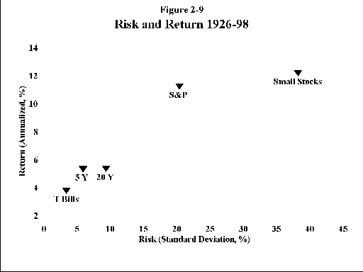
When it comes to US securities, we are sitting in clover: there is usable data going back to the birth of the Republic regarding common stocks and government bonds, and extremely detailed data going back to 1926. One of the great bargains in the investing world is the Ibbotson monograph, Stocks, Bonds, Bills, and Inflation (known in the investing world as "the SBBI"). This contains every possible breakdown for returns, risks, and correlations of a large number of US assets for periods ranging from 1 month to decades. We shall consider 5 assets: large and small US stocks, and 1-month, 5-year, and 20-year treasury securities. The below table summarizes the relevant data:

Asset	Annualized Return 1926-98 (%)	SD 1926-98 (%)	Worst return for a single year 1926-98 (%)	Return for 1929-32 (%)
1-Mo T-bills	3.77	3.22	0.00	+9.5
5-Yr Treas.	5.31	5.71	-2.65	+20.2
20-Yr Treas.	5.34	9.21	-9.8	+19.8
Large Stocks	11.22	20.26	-43.3	-64.2
Small Stocks	12.18	38.09	-58.0	-85.7

 

The data in the above table summarizes what you really need to know about US stocks and bonds in the aggregate—it would not be a bad idea to commit the approximate return and SD figures for the 5 assets to memory.

Let’s review each asset individually. You should refer to the series of graphs in the following pages for each asset. The terminology for government securities is confusing. A security of less than 1 year is called a "treasury bill," or more simply, "T-bill." An obligation of 1 to 10 years is called a "note," and of greater than 10 years a "bond."

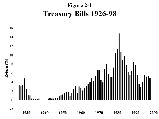
A. Treasury bills (Figure 2-1)—This is the safest investment on earth. Short of national destruction, there is no possibility of default, although Uncle Sam occasionally prints money to make good. The price paid for this safety is steep; the return is only 3.77%, which is barely above the inflation rate of 3.08% for the 1926-98 period. Further, although many academicians consider T bills to be "riskless" a quick perusal of the T-bill graph shows considerable variation of return, meaning that you cannot depend on a constant income stream. This risk is properly reflected in the SD of 3.22%. The best that can be said for the performance of T bills is that they keep pace with inflation in the long run, although there were prolonged periods when even this was not true, particularly in the 1970s.

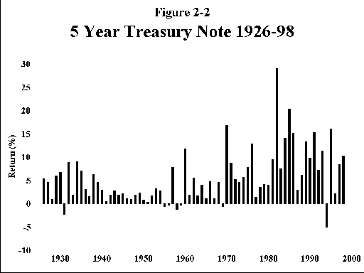
B. Intermediate term (5-year) treasury notes (Figure 2-2)—Like T bills, these instruments offer near absolute protection from default on principal and interest, but do carry one risk—that of rising interest rates. A note or bond yielding a fixed coupon will decline in market value when interest rates rise, and the longer the maturity of the note or bond the worse the damage. At a maturity of 5 years, the loss in principal market value can exceed the dividend yield of the note or bond, resulting in a negative total return for the year. This has happened 6 times in the past 73 years, and, in fact, the worst loss for this period (2.65%) occurred in 1994. For bearing this risk you are rewarded with another 1.5% of long-term return. In the long run, you can expect a real (inflation-adjusted) return of about 2%.

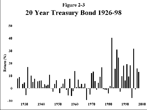
C. Long-term (20-year) treasury bonds (Figure 2-3)—These instruments behave in much the same way as the intermediate bonds, except that their interest rate risk is much worse, producing losses in 16 of the past 73 years, with 1 loss of nearly 10%, and many in excess of 5%. Surprisingly, you do not seem to be rewarded at all for bearing this risk; the return is almost identical to that for 5-year notes.

Why do many sophisticated investors invest in long bonds, when they can have the same return with less risk with intermediate bonds? In fact, there are many single assets whose apparent risk seems out of proportion to their meager returns. The best example of this is the class of precious metals stocks, with real long-term returns of a few percent, and an annual SD of about 30%. The answer, which we shall explore in later chapters, is that the "excess risk" of these assets disappears in a properly constructed portfolio. That part of the risk which disappears with diversification is called "nonsystematic risk," and that which remains and cannot be diversified away is called "systematic risk." (There is another reason why the returns on long treasuries are so low, having to do with the fact that they are a favorite investment of insurance companies, which have long-lived fixed liability commitments, which can be precisely offset with long bonds.)

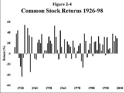
D. Large company common stocks (Figure 2-4)—This series consists of the various groups of large companies, or " indexes," for the past 73 years. The latest incarnation of this is the familiar S&P 500. The reader may find the terminology of this group confusing. They are referred to variously as "large stocks," "S&P," "S&P500," "common stocks," or simply as "stocks." For the purposes of this book all of these terms are interchangeable.

The rewards of this asset are considerable; a real return of greater than 8%. The lure of common stocks is undeniable—your inflation adjusted wealth will double every 9 years. Put away $10,000 for your newborn child, and in 50 years he or she will have $470,000 of current spending power for your grandkids’ college educations. This return does not come for free, of course. The risks can be stomach turning. The SD is 20.26% (This is the number behind Uncle Fred’s coin toss—its SD is also 20%.) You can lose more than 40% in a bad year, and during the 4 calendar years 1929-32 the inflation-adjusted ("real") value of this investment class decreased by almost two thirds!

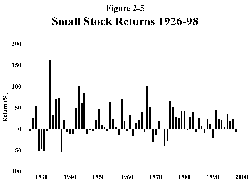
E. Small company stocks (Figure 2-5)—These are the stocks of very small companies, representing companies whose total outstanding stock value, or "market cap" places them in bottom 20% of the New York Stock Exchange by size. (In the current era most of these stocks are actually traded over the counter.) Here, the returns and risks are industrial grade. Your real return is now greater than 9%, meaning that you will double your money in inflation adjusted terms in just 8 years. Put away $10,000 for your grandkids and you will have $785,000 in 50 years in current spending power. But oh, the risks—for 1929-32 this investment class lost over 85%!

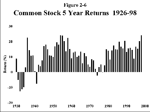
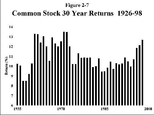
Figures 2-6 and 2-7 show the effects of longer holding periods for large company US stocks. Figure 2-6 shows rolling 5 year returns for large stocks; except for the period of the great depression, things do not look so scary, with only a few losing periods. The picture shown in Figure 2-7 for 30 year holding periods is positively tranquil; not a single 30 year period with a return of less than 8%! The message is clear; stocks are to be held for the long term. Don’t worry too much about the short term volatility of the markets; in the long run stocks will almost always have higher returns than bonds.

This subject can also be analyzed from a theoretical viewpoint. Using some relatively simple statistical methods, one can calculate the risk of underperforming the "risk free" T-bill investment. This method assumes a return on common stock of 10%, an S.D. of 20%, and a T-bill rate of 3%. In any given year the risk of stocks underperforming T-bills is 36%. For a 5 year period this risk is 22%, for 10 years, 13%, for 20 years, 6%, for 30 years 3%, and for 40 years it is only 1%. The message is the same; the longer one’s time horizon, the less likely the risk of loss.

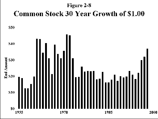
(A word of caution here. Some have interpreted the above data as demonstrating that "stocks grow less risky with time." This is not quite true. Take a look at Figure 2-7. The difference between the highest and lowest 30 year return is almost 5%. Compounding a 5% return difference over 30 years produces an almost 4-fold difference in end-wealth. Figure 2-8 demonstrates the vastly different end-wealths of $1.00 invested over the various 30-year periods since 1926. This plot shows that when you measure risk as the standard deviation of end-wealth, then stocks actually become riskier with time. This is not a trivial or theoretical distinction. Probably the most relevant definition of risk is the likelihood of running out of money. It is vitally important that you think about what measure of risk best describes your own personal needs and perceptions.)

 

EVERYBODY’S GRANDCHILDREN OUGHT TO BE RICH

In the halcyon early summer of 1929, John J. Raskob, a senior financier at General Motors, granted an interview to Ladies Home Journal. The financial zeitgeist of the late 1920’s is engagingly reflected in a quote from this piece:

 

Suppose a man marries at the age of twenty-three and begins a regular savings of fifteen dollars a month—and almost anyone who is employed can do that if he tries. If he invests in good common stocks and allows the dividends and rights to accumulate, he will at the end of twenty years have at least eighty thousand dollars and an income from investments of around four hundred dollars a month. He will be rich. And because anyone can do that I am firm in my belief than anyone not only can be rich but ought to be rich.

Mr. Raskob’s hypothetical young man was an investment genius indeed—turning 15 dollars per month into $80,000 in 20 years requires an annualized rate of return of over 25 percent. This interview, and the investment scheme he was promoting, is remembered to this day as an absurd example of the infectious mood underlying the pre-1929 stock bubble.

And yet, in the long run Mr. Raskob was not far off the mark. Let’s imagine that Mr. Raskob’s hypothetical young man began investing 15 dollars per month in common stocks on January 1, 1926 and continued doing so until he died at age 91 on December 31, 1994. By that date he would have accumulated $2,462,295. Had he invested in small stocks, he would have $11,730,165. Obviously, this calculation contains a number of unrealistic assumptions: that the principal and dividends were never spent, taxes were not paid, and stocks were bought free of commissions. Perhaps our estimates are off by a factor of 2 or 3; still, the long-term results are impressive.

An optimist might cite this as an example of the "magic of compound interest." Too much is made of this phenomenon. A pessimist would note that our industrious saver died an old man without enjoying his fortune; had he consumed even a few percent of it each year his estate would have been vastly smaller. Personally, I’d rather be a 26 year old roaming the boulevards of Paris with a few francs in my pocket than a rich old man. Everyone cannot be rich, but perhaps their grandchildren can.

I urge you to spend a few minutes perusing Figures 2-1 to 2-8, and to impress yourself with the magnitude of the risks involved in bonds and common stocks. The next 73 years will likely be just as bumpy as the last.

Individual investors are inevitably drawn into stocks during powerful bull markets; the spectacle of one’s friends and neighbors achieving quick and effortless wealth awakens the powerful forces of human nature. Those sucked into the market for the first time during such enthusiasms invariably lack a proper appreciation of the risks associated with high returns; they draw comfort from the blandishments of experts that they can "keep close to the exits" and sell their stock the moment the bear growls. After they have suffered the inevitable losses, they are overcome by an even more powerful element of human financial nature; the urge to psychologically distance themselves from their "failure" and thus sell at a great loss, usually when prices are the lowest. The plain fact of the matter is that no investor, no matter how skilled, ever avoids bone crushing losses at times even when undertaking the most prudent market risks. All investors, novice and experienced alike, are well served by the words of John Maynard Keynes:

I do not feel that selling at very low prices is a remedy for having failed to sell at high ones.... I feel no shame at being found owning a share when the bottom of the market comes. I do not think it is the business, far less the duty, of an institutional or any other serious investor to be constantly considering whether he should cut and run on a failing market, or feel himself to blame if shares depreciate on his hands. I would go much further than that. I would say that it is from time to time the duty of the serious investor to accept the depreciation of his holdings with equanimity and without reproaching himself...(italics mine) An investor is aiming, or should be aiming, primarily at long term results, and should be solely judged by these. The fact of holding shares which have fallen in a general decline of the market proves nothing and should not be a subject of reproach.

Fortunately, there are ways to lessen the raw risks of single assets, and there are often times when the addition of a small amount of a very risky asset to your portfolio will actually lessen its volatility.

ASSETS CLASSES IN THE 1970-98 PERIOD

The previously discussed 1926-98 database for US assets provides a reliable estimate of the expected long term return and risk in US stocks and bonds. In fact, there is data on the long term returns and risks of these assets going back 200 years, albeit considerably less detailed and accurate; the inflation adjusted returns and SDs data are very similar to the 1926-98 data. (For an excellent discussion of stock returns throughout the entire history of the US, see Siegel’s Stocks for the Long Run.)

Unfortunately, the 1926-98 database is confined to US equities and high quality bonds, and is thus much too limited to be of real use to the modern investor, who has available a much wider variety of capital markets to choose from. There is great advantage to be gained from wide diversification among as many potential investment categories as possible. All investors, small and large, require accurate estimates of the returns and risk of each of these investments. I have chosen 1970 as the starting point for this expanded database, as high quality data are available from this date for a wide variety of assets. 1970 was also chosen as it forms an important watershed in investment history—the bear market of 1973-4 was the worst experienced by the capital markets globally since the great depression. It is instructive to include the performance for these 2 years for each asset as a guide to their risk. It is also useful to have such a ferocious bear market included in any consideration of asset return as a vigorous dose of "reality testing." This database also has one further advantage—it is almost completely accessible from a wide variety of sources, such as Morningstar products, for a nominal fee (see Chapter 9 for further details).

 

ASSET PERFORMANCE FROM 1970 TO 1998

ASSET	RETURN	RISK(SD)	WORST YR	1973-74
T-bill	6.76	2.61	+3.00	+15.48
5 Yr Treas	9.03	6.62	-3.58	+10.56
20 Yr Treas	9.66	11.58	-7.78	+3.20
S&P	13.47	15.94	-26.47	-37.25
REIT	13 ?	17 ?	-21.40	-33.58
US Small	13.62	22.58	-38.90	-56.44
European Stocks	13.63	20.30	-22.77	-28.74
Pacific Rim Stocks	9.69	31.23	-50.59	-54.80
Japanese Stocks	12.61	33.49	-36.18	-27.65
Precious Metals Stocks	10 ?	43 ?	-41.51	+112.83
International Small Stocks	16.98	31.22	-28.61	-38.38

(Source: Ibbotson Associates, NAREIT, Morgan Stanley Capital Indexes, Dimensional Fund Advisors)

You have already encountered T-bills, 5-year notes, 20-year bonds, the S&P stocks, and small US stocks in the 1926-98 database. Real Estate Investment Trusts (hereafter referred to as REITs) are companies which derive their revenue from the management of commercial property. I have excluded those REITs which derive their income primarily from mortgage activity, and include only so-called "equity REITs." The European, Pacific Rim, and Japanese stock indexes derive from the Morgan-Stanley Capital Indexes, and represent the largest stocks in those markets. Precious metals stocks represent the gold and silver mining industry. Finally, international small company stocks are the foreign equivalent of the US small stocks. This index is kept by the Dimensional Fund group, and care is urged in its use, since before 1988 it constituted only two countries, the UK and Japan.

Casual perusal suggests that returns for the 1970-98 period are higher than for the 1926-98 period (about 4% higher for the 3 bond categories, 1.5% for small stocks, and 2.5 percent for large stocks). However, inflation for the recent period was 5.23% annualized versus 3.1% for the 1926-98 period, so real returns were about the same for large stocks, smaller for small stocks, and higher for all the bond categories. Comparing the tables for the 2 periods also suggests that the 1929-32 bear market was much worse than the 1973-4 market. Again, this is largely illusion, as the 1929-32 bear market was characterized by severe deflation, and the 1973-4 market by severe inflation. In real terms, the 1929-32 market was only slightly worse than the more recent one for large stocks.

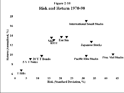
As with the 1926-98 database, there is a good correlation between risk and reward, with 2 notable exceptions—precious metals stocks and Pacific Rim Stocks, whose returns were not commensurate with their risks. Note the question marks after the returns of both REIT and precious metals stocks. There are no easily available data regarding these asset classes. To estimate the long-term returns for precious metals stocks I used the Morningstar mutual fund objective data, which goes back to 1976. For the years 1970-75 I used the returns of a "proxy" mutual fund—the VanEck Gold Fund. For REITs I used data from the National Association of Real Estate Investment Trusts (NAREIT), which extends back only to 1971. The makeup of the REIT sector has undergone dramatic changes in the past 5 years, and the historical NAREIT returns may no longer be representative. The long-term returns data for both of these areas is highly suspect, and should not be used for planning purposes. However, even if the returns of these two assets were very low, many investors may still want exposure to them. The main reason for this is that they are perceived to be inflation hedges, and likely to do well in an inflationary environment in which other stocks and bonds would be adversely affected. This is the same as saying that much of the risk of precious metals and REITs can be "diversified away." More about this later.

Figures 2-9 and 2-10 display return/risk plots for the 1926-98 and 1970-98 asset bases. For each asset the risk, quantified as the SD, is plotted along the horizontal axis (also known as the "x axis"). Safe assets are clustered on the left side of the graph; as we move off to the right, risk/SD increases. Annualized return plotted along the vertical axis (also known as the "y axis"). As we move from bottom to top, return increases. Note how for almost all assets, as return increases, so does risk. If we were to draw an imaginary line through the points it would slope up to the right; most assets lie on a fairly straight line, showing clearly the direct relationship between risk and reward. The 2 major exceptions to this are precious metals and Pacific Rim stocks, as noted above.

THE PROBLEM WITH HISTORICAL RETURNS

One area which gives even finance professionals real problems is the estimation of future asset returns. One expedient is simply to use historical returns, and the quality and detail of the available data, particularly from Ibbotson, makes this particularly attractive. Most analysts learn from hard experience, however, that it can be hazardous to blindly extrapolate past returns into the future. It is extremely helpful to have an intuitive idea of how to estimate the future returns of stocks and bonds.

Long bonds are relatively easy. A good approximation of their return is simply the coupon. Say you have a 6% 30-year Treasury bond. If interest rates do not change, you will in fact receive a 6% long-term return. If rates fall, then you will obtain a slightly lower return, as the coupons will be invested at a lower rate (so-called "reinvestment risk"). If rates rise, the opposite will occur. Still, even with significant long-term bond market volatility the long-term return will not be more than a few percent off the coupon rate. At the beginning of 1926 the coupon on long-term AAA corporate bonds was 4.9%—not too far off the actual return for 1926-98 of 5.77%.

Long bonds also nicely illustrate the dangers of relying on historical returns too heavily. From 1958 through 1983 bonds underwent a brutal, grinding bear market, as long-term treasury rates rose from less than 3% to over 14%. (Bond prices move in the direction opposite coupon changes.) Because of this, the annualized returns of 20-year Treasury bonds for the 50-year period from 1934 to 1983 were only 3.5%, which was actually slightly less than inflation. Had you relied on this historical return you would have come up with a ridiculously pessimistic estimate of future returns in 1984. As it turns out, in 1984 the 14% coupon more accurately forecasted the 12.85% returns over the subsequent 15 years. (The lower annualized return resulting from the fact that the coupons had to be reinvested at an ever-falling rate.) As this book is being written long Treasuries are again yielding a reasonable 6%, so their expected return should be close to the historical 5% norm.

Stock returns are not so easy. Probably the most time honored method of estimating future stock returns involves the so-called "discounted dividend" method. It goes something like this; over a long enough time period, all companies go bankrupt. (Take a look at the stock page from the Civil War and you will find that almost none of the names are recognizable.) The value of a stock thus comprises the "discounted" value of all of its future dividends. (We'll discuss in Chapter 7 just how to go about doing this sort of calculation.) If you were a Rip vanWinkle investor who invested $10,000 in the stock market and then went to sleep for 200 years, all you would be left with when you awoke would be generations of reinvested dividends from a long list of mostly defunct companies. (Mind you, this would be a very large amount of money.) Estimating the value of a stock or stock market by this method is a very complicated calculation, but can be simplified as follows:

Long-term return = dividend yield + growth rate + multiple change

Since 1926 stocks actually yielded an average of about 4.5%. Earnings and dividends have grown at about a 5% rate. And stocks which once sold for 10 times earnings in 1926 now sell for 30 times—this calculates out to an annualized multiple change since then of about 1.5%. Add these 3 numbers together and you get 11%, compared to the actual historical return of 11.22%. Not too shabby. (There were, of course, a few bumps on the road to that return.)

Unfortunately, as we start the millennium, things look a little different. The current dividend yield of the S&P 500 is about 1.3%. Economic growth is still about 5 percent. And the prudent investor should not expect any further expansion of earnings and dividend multiples. Adding the two numbers gives an expected return on common stock of only about 6.3%, versus the 6.0% percent coupon on long bonds. Thus, over the next few decades, stock returns should be only slightly higher than bond returns.

Simply put, the current optimism surrounding stock investing does not appear to be well founded. (In fact, in 1998 the expected returns of corporate bonds calculated in this manner briefly exceeded that of stocks.)

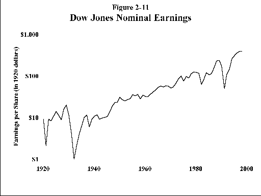
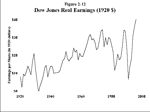
The famous financial analyst, Benjamin Graham, once said that in the short run the stock market is a voting machine, but that in the long run it is a weighing machine. What it weighs are earnings. In these ebullient times, the torpid and occasionally stuttering growth of common stock earnings cannot be stressed strongly enough. For this reason I’ve plotted the earnings of the Dow Jones Industrial Average from 1920. Figure 2-11 shows earnings in nominal dollars, with no adjustment for inflation. The plot slopes upward at about 5% per year. Figure 2-12 shows the same data in inflation adjusted dollars, relative to the value of a dollar in 1920. (To convert to 1999 dollars, multiply by 9.) It slopes upward at only about 2% per year. It is illogical to expect the value of a broad index of US stocks to significantly exceed this "natural" 5%/2% nominal/real growth rate. To this return can be added your dividends. To expect more is folly.

It is more difficult to perform a similar analysis for other asset classes. It appears that the expected returns of European and Japanese stocks should be about the same as for US stocks. US small stocks should have somewhat higher returns. Pacific Rim and emerging markets stocks currently yield about 3%-4%, and may have growth rates higher than in the US, and thus may have higher returns—but of course with much higher risk. The greatest anomaly of all, however, are with REITs, which are currently yielding an almost unbelievable 8.8%. Even if they experience no earnings growth, their returns should be higher than the S&P 500.

And, to round things off, the T-bill return is almost impossible to forecast, since its "coupon" (Strictly speaking, it has none, as T-bills are sold at a discount and mature at par.) changes from month to month.

So, as the famous test pilot Chuck Yeager would say, we’ve got a little problem here. Our stock return predictions from the discounted dividend model are considerably lower than historical returns. What is the intelligent investor to do?

There is no right answer to this dilemma, but I would err on the conservative side and go with the discounted dividend model. Using this method, it should be possible for you to calculate your long-term expected investment return based on your investment choices, or "asset allocation policy." You should also be able to estimate the risk that you are taking in order to achieve this return.

As already alluded to, the most useful way to estimate your expected return is as inflation adjusted, or "real" return. This will in turn simplify your retirement calculations, as the effects of inflation have already been discounted. Projecting a 4% stock return in real dollars is easier than projecting a 7% nominal return, then adjusting for a 3% inflation rate, particularly when your withdrawals may be spread over 15 to 30 years. So, here is the bottom line:

 

Asset	Expected Inflation- Adjusted Return	Worst Bear Market Loss
T-bills	0-3%	None
All other high quality bonds	3%	None(Short duration) 10%(Long duration)
Large company stocks, US and foreign	4%	40-50%
REITS, Small company stocks, US and foreign, emerging markets stocks	6%	50-60%
Precious Metals Stocks	0-4% (???)	50-60%

This table provides a handy back-of-the envelope way to plan your finances. You say you can tolerate a 25% bear market hit as long as it occurs only once in your life? Fine. Looking at the last column, we see that a portfolio consisting of about 50% stock, split between large and small companies, and the rest bonds of short duration, will lose about 25% in a once-in-a-lifetime bear market. Your real (inflation-adjusted) portfolio expected return can be calculated as follows:

1. 25 percent of your portfolio is in small stocks. .25 x 6% = 1.5%

2. 25 percent of your portfolio is in large stocks. .25 x 4% = 1.0%

3. 50 percent of your portfolio is in bonds. .5 x 3% = 1.5%

Thus, the real long-term expected return of your portfolio is:

1.5% + 1.0% + 1.5% = 4.0%. This means that you will about double the real value of your portfolio every 18 years. (This is easily calculated from "the rule of 72," which says that the interest rate times the doubling time of your assets should multiply out to 72. In other words, at 6% return your capital will double every 12 years.)

Take another break. Don’t look at this book for at least a few more days. In the next chapter we shall explore the strange and wondrous behavior of portfolios.

CHAPTER 2 SUMMARY

1. Risk and reward are inextricably intertwined. Do not expect high returns without high risk. Do not expect safety without correspondingly low returns.

2. The longer a risky asset is held, the less the chance of a poor result.

3. The risk of an asset or a portfolio can be precisely measured. The easiest way to do this is by calculating the "standard deviation" of returns for many time periods.

4. Those who are ignorant of investment history are bound to repeat it. Historical investment returns and risks of various asset classes should be studied. Investment results for an asset over a long enough period (greater than 20 years) are a good guide to the future returns and risks of that asset. Further, it should be possible to approximate the future long-term return and risk of a portfolio consisting of such assets.

 

copyright (c) 1999, William J. Bernstein