Rolling Your Own: Three-Factor Analysis

If you’re responsible for overseeing a gazillion dollars of pension money, it’s not enough to open up the quarterly mutual fund supplement of your local paper and compare your manager to her peers or the indexes. The reason is simple: you really don’t know whether her good/poor performance was due to a lucky/unlucky style tilt in her security selection. Maybe her large-growth top-heavy bias added several percentage points to her returns, but beyond that she couldn’t pick a stock out of a hat if her life depended on it. How do you correct for these biases? The best way to do so is to use a "factor-based analysis" (FBA). FBA is to active money managers, what a light switch is to cockroaches.

There are as many different kinds of FBA as there are portfolio analysts, but the simplest, best known and probably most powerful is the so-called "three-factor model" (3FM) of Fama and French. In April 1999, I touched on this method in an article on small-growth investing, but didn’t provide a lot of details. The reason was, the returns series necessary for these calculations were not yet in the public domain.

Now, thanks to Ken French’s wonderful online data library, the 3FM is available to the small investor for the analysis of manager returns. The "Fama-French Research Data Factors" file contains the monthly and quarterly returns for the four necessary data series:

• The 30-day T-bill return
• The return of the total market (CRSP 1-10) minus the T-bill return (Mkt)
• The return of small company stocks minus that of big company stocks (Small minus Big, or SmB)
• The return of the cheapest third of stocks sorted by price/book minus the most expensive third (High minus Low, or HmL)

Once you have the returns series for the manager you want to look at, you’re on your way. Here’s the cookbook:

1. First, you need a spreadsheet package capable of performing multiple regression. In this day and age, it means being conversant with Microsoft Excel. (If you need help with either statistical analysis or Excel, John Neufeld’s old Learning Business Statistics with Microsoft Excel series is excellent, even though the last edition is more than a decade old; Excel really hasn't changed enough to detract from its value.

2. Next, you need to download from  the regression seriess from Professor French's site. (Note: this is a zipped text file, which you'll have to decompress and import into csv/xls/xlsx format.) 

3. Third, you need to extract the monthly returns for your money manager. This is the tricky part. Ideally, you’ll have Morningstar Principia Pro Plus, but even then the extraction process is not completely painless. You have to output the monthly returns from the Advanced Analytics section (Risk and Reward/Rolling Return - Table, and make sure you select the one-month rolling period). Then, once you’ve opened this in Excel you need to use the copy/edit/paste special/transpose sequence to get it into vertical format. And if you only have the plain-vanilla Principia Pro package, you’ll have to extract the monthly returns point-by-point with the graph function.

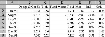
   Lay this series next to the T-bill returns, and subtract the latter from the former. You now have a column that represents the difference between the two, which is the "risk-adjusted return" (RAR). As an example, I’ve chosen the Dodge and Cox Stock Fund. Column B contains the raw returns; column C, the T-bill returns; column D, the RAR (column B minus column C); and columns E, F, and G, the three regression series. The six rows of the spreadsheet should look something like this:

   

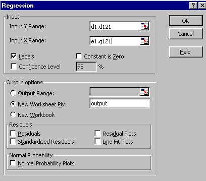
4. Last, multiply regress the RAR versus the Mkt, SmB, and HmL series. I recommend including the labels in the regression menu.

Here’s what the regression dialog box looks like:

Note that I’ve started the regression in row 1, where the labels are, and checked the "label" box. Finally, the abbreviated output is shown below:

Regression Statistics
Multiple R	0.9118679
R-Squared	0.8315031
Adjusted R-Squared	0.8271454

	Coefficients	Standard Error	t-Stat	p-Value
Intercept	-0.2058513	0.1590456	-1.2942908	0.1981357
Mkt	1.0575511	0.0450486	23.475762	6.991E-46
SmB	-0.0538972	0.0453912	-1.1873937	0.2374981
HmL	0.4876222	0.0638117	7.6415827	6.747E-12

 

The first group of statistics shows us that we have a fairly decent fit with the data, with a raw R-squared of 0.91. This tells us that 91% of the fund’s monthly returns are explained by the three factors.

The second group is far more interesting. First, the "intercept" is the fund’s alpha, negative 0.206 per month, or about 2.5% per year. In other words, the managers, after expenses, underperformed the regression-based benchmark by that amount. However, the t-stat and p-value tell us that this is not statistically significant. Next, we have the "loadings" for the three factors. The Mkt loading is 1.06. This is the traditional beta of the fund. Most equity-only funds have values very close to 1.0. The SmB loading is -.05. This means that the fund is primarily large cap. (A zero value signifies large cap, and a value of greater than 0.5, small cap.)

Finally, the HmL loading is 0.49, which tells us that we’re looking at a value fund. (A zero value defines a growth portfolio, a value of more than 0.3, a value fund.)

A fourth factor, momentum, can also be thrown in, as can many others. You cannot overestimate the power of this model. Wirehouse reps and pension consultants are fond of "attribution analysis," which usually consists of qualitative excuses for a manager's lackluster performance in a given period. The 3FM throws investment results into much sharper relief. Let me give you a real-life example:

I sit on a committee overseeing a local institution's pension portfolio and was treated to our consultant's sheepish exposition of our small-cap fund's obviously dismal performance. But when its returns were tossed into the 3FM grinder, a stunning picture emerged: market and size loadings of 1.0, a value loading of zero, an R-squared of 0.99, and an alpha of minus 10% per year. In other words, we had been burned by a manager doing his best to mimic the CRSP 9-10 index (which has almost identical loadings), but who couldn't transact his way out of a paper bag.

Unfortunately, positive prior alpha does not predict future positive alpha. Robert Sanborn of Oakmark Fund manufactured spectacularly positve results in his first few years, only to achieve similarly spectacular negative results just before he "retired."

As should be evident from the above methodology, this technique is not for the faint-of-heart. Even with my fingers flying, the export-transform-import-regress cycle required usually takes about ten minutes for each fund. But master it and you've gone most of the way toward minimizing your chances of being sandbagged by a consultant or manager.

Copyright © 2001, William J. Bernstein