- Increased by the volatility of each asset
- Increased by a decreased correlation between each asset,
- Decreased as the difference in long term returns increases, and
- Decreased further if this return difference is maintained over a long period of time
![]()
When Doesn't It Pay to Rebalance?
William J. Bernsteinwbern@mail.coos.or.us
Perold and Sharpe point out that rebalancing is a "concave" strategy. Portfolio insurance represents the opposite of rebalancing, and is referred to as a "convex" strategy. They suggest that convex portfolio insurance strategies as well as buy and hold ("flat") strategies produce superior returns in markets with a prolonged upward (or downward) bias, and concave rebalancing strategies produce superior returns in stagnant markets. If the only two assets considered are stocks and bonds, and if stock returns are always much higher than bond returns over long time horizons, then obviously buy and hold, as well as portfolio insurance, will produce returns superior to rebalancing. As already pointed out, this will come at the cost of gradually increasing portfolio risk.
However, things are very different for global equity portfolios. Over very long time horizons there is usually relatively little difference in the returns in most national equity markets; under such circumstances rebalanced portfolios dominate. For example, when looking at the 1970-94 period, rebalancing various MSCI national asset pairs almost always provides returns superior to nonrebalanced national pairs. Only when long term return differences among asssets exceed 5 percent do nonrebalanced portfolios provide superior returns, and then only at the cost of increased risk. (The exceptions which prove the rule are the very high returns of Japanese equity, and the very low returns of Australian and Italian equity.) Care should be taken to note that the superiority of rebalancing as a long term strategy pertains only to national and regional markets as a whole, and not among different industry groups. Over the course of decades entire industries often shrivel while others prosper mightily; rebalancing the pharmacutecal and petroleum segments of the S&P500 over the past three decades would have been a disastrous strategy. Although enitre national markets occasionally disappear throught war or nationalization, this occcurs much less frequently than the ongoing remolding of market segment capitalization characteristic of a market economy.
In last month's Efficient Frontier we derived the following formula, which was found to accurately predict the RB, defined as the return in excess of the Markowitz return calculated from annualized data:
or more simply,
Stated succinctly, the intrinsic rebalancing potential of any asset pair is the difference between its mean variance and covariance. However, the RB calcualted from the above formula is valid only when returns for the assets involved are similar. How dissimilar do asset returns have to be before it no longer pays to rebalance? Obviously, over the 69 year period for 1926-94, the 4.68% difference between stocks and corporate bonds is "too high" to produce a rebalancing benefit in terms of return alone, although rebalancing still produces benefits in terms of risk reduction.
It is clear from the above that the actual rebalancing bonus of a two asset portfolio is:

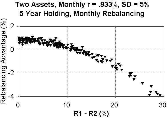
For a 5 year holding period, the following plot was obtained:

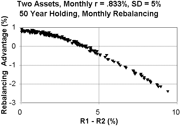
So, for a 50/50 mix of two assets with the approximate risk/return characteristics of US common stock and a zero correlation (as occurs with randomly generated returns) the "break even point" occurs at about 4% annualized return difference over a 50 year period, and about a 12% annualized return difference over a 5 year period. In other words, if the return gap between these two noncorrelated assets is less than 4% annualized over 50 years, or less than 12% over 5 years, then it pays to rebalance. If the return gap is greater, it does not.
For those of you who are interested, I've plotted the results for the following asset pairs:
Both Assets monthly r = 0.00833, monthly SD = 0.05
(above example)
Both Assets monthly r = 0.01, monthly SD = 0.1
(simulates a pair of very volatile stock classes
e.g., precious metals and emerging markets stocks)
One asset monthly r = 0.00833, monthly SD = 0.05
Second asset monthly r = 0.004167, monthly SD = 0.02
(Stock/Bond Model)
The data from the above graphs is tabulated below. Break even points for each model and holding period are estimated from the graphical data:
| .00833/.05 Model | .01/.1 Model | .00833/.05- .004167/.02 Model | |
| 50 years | 4% | 5.5% | 3% |
| 20 years | 6.5% | 13% | 5% |
| 10 years | 8% | 17% | 7% |
| 5 years | 12% | 23% | 9% |
Discussion
The above simulations provide an approximate answer to the question "Under what circumstances does it pay or not pay to rebalance?" Rebalancing works best with volatile, uncorrelated assets whose returns are roughly similar. The above table of break even points provides an "outer limit" beyond which rebalancing is of no benefit. In the real world of the global equity markets, correlations among different national indexes average about 0.5. This would necessitate adjusting the above values down by about a third. Transaction costs will result in further downward adjustment, and taxability may completely eliminate any rebalancing benefit at all.Consider for a moment that almost all of the world's major equity markets have monthly standard deviations clustering between the .00833/.05 and .01/.1 models used above. Over a 20 year period one can estimate the zero correlation break even point at about a 10% annualized return difference. Taking into account transaction costs and nonzero correlations an actual break even point in the 5%-6% range seems reasonable. How likely is it that the average difference in 20 year annualized return among various national or regional markets will be this large? Not very likely, in my opinion.
The above data also sheds some light on the stock/bond rebalancing problem. The last column of data in the table provides break even points for 2 assets with return/SD of .00833/.05 and .004167/.02. These are the approximate values for stocks and bonds. Over a 20 year period, the rebalanced portfolio will dominate if the annualized return difference is less than 5%. The expected long term return of common stocks at current prices can be closely approximated by the discounted dividend model at about 7% (2% dividend yield plus 5% earnings/dividend growth). This is about the same as the expected return of long term corporates, which is reasonably approximated by their current yield. If you believe that that stock returns over the next few decades are going to be 5% greater than long term corporate returns, then I have a large expanse of steel and concrete connecting Manhattan and Brooklyn that I can sell you which will provide you with an excellent cash flow in your old age.
One must decide whether or not to rebalance one's portoflio. The above framework provides a rational quantitative framework in which to make this decision.
William J. Bernstein
wbern@mail.coos.or.us
![]()
![]()
copyright (c) 1996, William J. Bernstein
